CS 6362 - Advanced Machine Learning

Assignment 5

In this assignment you will extend your sparse variational GP from assignment 4, and train the model to set the GP hyperparameters. Specifically, your objective is to find hyperparameters that maximize the variational lower bound on the log marginal likelihood. Optimization will be performed through gradient ascent on the lower bound.

JAX

As part of gradient-based learning, it will be necessary to compute derivatives of the lower bound with respect to kernel parameters. Rather than hand-deriving these derivatives, you will use JAX, a library designed for reverse-mode differentiation.

You can view JAX as a lightweight PyTorch or TensorFlow: the ability to compute derivatives based on computation graphs built up from your code, but without all of the bells/whistles/overhead of a machine learning library.

You will only need to use a very small number of features of JAX for this assignment – see appendix below for a few other details.

1. JAX has most of the functionality of NumPy. Using JAX is as simple as replacing your import numpy as np code with import jax.numpy as np. Likewise, for scipy, you would replace import scipy.linalg with import jax.scipy.linalg. Arrays, and their operations, remain the same. The only difference between NumPy arrays, and JAX arrays, is that JAX arrays are immutable. That is, you cannot slice existing arrays to assign new values.
2. The primary use of JAX for this assignment is to compute derivatives. Please see the following references for examples: example 1, example 2. Thus, it will be required to have a dedicated function for computing the lower bound log marginal likelihood, which takes in as its first argument hyperparameters that you are trying to find. Gradients will then be computed with respect to these parameters – for convenience, this can be a dictionary of key:value pairs, one per parameter. This function can have other arguments too, but gradients for these arguments will not be computed.

Gradient ascent of the lower bound (50)

To optimize the lower bound, you will implement gradient ascent. You will need to be careful in setting up the optimization problem:

1. Initialization: the hyperparameters will need to be initialized to … something. As I recommended in the previous assignment, for length scales (if you are using squared exponential kernels), per-feature statistics are useful here. I suggest initializing length scales to some multiple of their standard deviation, in order to get the scale within a reasonable range. Otherwise, you will likely end up in undesirable local maxima.
2. Noise variance, signal variance: if you did not consider these hyperparameters, you definitely should in this assignment. Signal variance, in particular, is an amplitude applied to the kernel (or if you are, say, summing multiple kernels, one signal variance per kernel). Initialization of these parameters is also crucial – I recommend setting both to 1 for simplicity.
3. Gradient ascent setup: here you should implement gradient ascent with momentum. There are 3 parameters you will need to set: the learning rate, the momentum parameter (a value between $[0,1]$), and the number of steps to take. Further, as we discussed, to ensure convergence you should slowly decay the learning rate over training, e.g. at the end, the learning rate should be 0. Consider a linear decay schedule.

The above should be done for a fixed set of inducing variables.

Optimizing for parameters and inducing variables (30)

Next, you will explicitly optimize for the inducing variables. To this end, the criteria you will use for selection – selecting a point(s) in the training set – is the trace term. Recall the lower bound from the Titsias paper:

$L_V = \log \mathcal{N}(\mathbf{y} ; \sigma^2 I + Q_{nn}) - \frac{1}{2 \sigma^2} tr(\tilde{K})$,

where $\tilde{K} = K_{nn} - K_{nm} K_{mm}^{-1} K_{mn}$, matrix $K_{nn}$ is the kernel evaluation between all pairs of training points, $K_{mm}$ is the kernel evaluation between all pairs of inducing points, and $K_{mn}$ is the kernel evaluation between inducing points and training points ($K_{nm}$ is the opposite).

You will develop an algorithm for alternating between (1) optimizing the lower bound parameters, and (2) selecting informative inducing variables. Specifically:

1. Initialize inducing variables from a small (e.g. 30) set of points from the training set.
2. Optimize the lower bound: here you should ensure that you take enough steps with gradient ascent.
3. Select a small (e.g. 10 or so) set of points that most reduces the trace ($tr(\tilde{K})$). Evaluating the trace can be expensive, so here you should derive an algorithm that balances (1) quality of points and (2) speed. Justify your algorithmic decisions in your report (see below).
4. Given the inclusion of the new inducing variables, perform gradient ascent. In comparison to Step 2, you should not need to take as many steps in gradient ascent.
5. Go back to step 3, until you have found a prescribed number of inducing variables.

Analysis (20)

You should prepare a PDF write-up as part of your submission that addresses the following:

Balanced Training

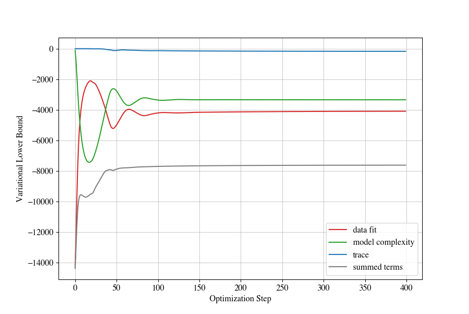
As part of maximizing the lower bound with a fixed set of inducing variables, plot the (1) data fit, (2) model complexity, and (3) trace terms associated with the log marginal likelihood over the course of training, as well as their sum. The purpose behind plotting this is to verify that your optimization is balancing data fit and model complexity. See, e.g., the following plot:

You should put together these types of plots for a small subset of the training data (e.g. $1000$ samples), and varying number of inducing variables (e.g. $100, 200, 500, 1000$). Note that when the inducing variables are identical to the full training data, then the lower bound becomes tight, and the trace term vanishes.

Point Selection Justification

Provide details on your point selection procedure, and justify the decisions that you made.

Comparison

Provide a quantitative comparison, measured in terms of (1) root mean square error evaluated on witheld data and (2) the log marginal likelihood bound, between the following options:

• No optimization: decide on a fixed set of hyperparameters, and fixed set of inducing variables.
• Optimize kernel parameters only: draw a random set of inducing variables and fix them, optimizing only for the kernel parameters.
• Full optimization: perform the alternating optimization scheme to find, both, kernel hyperparameters and inducing variables.

You should perform these quantitative analyses varying the training set size, and varying the number of inducing variables, similar to the previous assignment.

Found Hyperparameters

You should report on the hyperparameters found through training. In particular, which hyperparameters changed the most? What length scales seemed “important”? Here you may want to compute how much the length scales changed from their initialization, e.g. their ratio.

Suggestions

JAX tips

With very high probability you will require 64-bit floating point precision for your computations, namely, for computing the Cholesky factorization. Otherwise, numerical precision limitations will result in matrices that are not positive-definite. By default, JAX works in 32-bit floating point precision. To enable 64-bit floating point precision, at the very start of your code, issue the following:

from jax.config import config
config.update("jax_enable_x64", True)

Additionally, by default gradient computation in JAX assumes that the function that you aim to differentiate only returns a single value, namely a single scalar. You will very likely find it useful, for both debugging purposes and for the analysis above (“Balanced Training”), to return multiple values. To enable this, in your grad call, simply pass in the optional argument has_aux=True, see e.g. this reference.

Start Small

This assignment does not require that much code to be written. Nevertheless, you want to be incremental in how you approach this assignment. Some recommendations:

1. Ensure that you have a solid understanding of how to use JAX to compute gradients. Start with a toy example, then consider how your kernel hyperparameters can be treated as variables that are the central focus of differentiation.
2. Note that JAX should not require you to redesign your existing code. Your object-oriented approach to sparse variational GPs, e.g. representing your kernel as a class, poses no problems for using JAX.
3. For gradient ascent, I recommend logging all details to make sure that optimization is working, and stable. This includes the log marginal likelihood, and per-parameter partial derivatives.