CS 6362 - Advanced Machine Learning
Assignment 3
In this assignment you will implement a multi-class Gaussian process classification model, using the Laplace approximation. Please go here for data, and starter code.
Data
You are provided 2 datasets, one that is intended for debugging purposes and to gain some intuition for the model, while the other is a more realistic dataset.
The first dataset, found in data/points.json, is a set of 2D points, and each point is classified into 1 of 3 labels. Provided is a means of plotting the classification results, and consequently, the decision boundary (boundaries) learned by the model. Please refer to the simple_tester.py script for further details.
The second dataset is a dataset of image-based features, namely, representations from a pre-trained neural network, subsequently projected to 256 dimensions via PCA. The images are originally from the CUB Dataset, a dataset of fine-grained bird categories. Included are images from 15 different categories. Please refer to the cub_gp.py script for further details.
Multi-Class Laplace Approximation
A scaffold for implementing the Laplace Approximation has been provided in laplace_approx.py. It is recommended to build off of the structure, but not necessary.
In implementing this technique, assessment will be performed based on the following:
Finding the Posterior (40 points)
You will first need to implement Newton’s method. For multi-class classification, this requires the following:
- A specification of the Gaussian process, e.g. the covariance function. Note: this should be a multi-class Gaussian process, e.g. one covariance function per class. Latent functions of different classes are assumed independent of one another. It is recommended to build off of the kernel you implemented in Assignment 2, and extend it to handle the maintenance of multiple kernels, each comprised of distinct parameters. (10 points)
- Computation of the posterior, its gradient, and its Hessian for iteratively updating the mode. Specifically, you will need to perform Hessian-gradient matrix multiplication. As we discussed, a naive approach to this is not scalable, particularly for the CUB dataset you are provided. Hence, you are required to use the derivation based on the Woodbury matrix identity, please see Appendix below for details. (30 points)
Compute the Averaged Predictive Probability (40 points)
For a given set of test data, you should be able to compute their averaged predictive probabilites. Specifically:
- You should form the predictive mean for the latents, e.g. integrating out the posterior and the test likelihood. (10 points)
- Form the predictive covariance for the latents. At this stage, this will provide you with a multivariate normal distribution specific to the given test point. (20 points)
- Given this distribution, perform Monte Carlo integration to compute the averaged predictive probability: this will result in a discrete distribution over classes. (10 points)
No Model Selection
Hyperparameters have already been provided for you in the starter code. You do not need to concern yourself with model selection in this assignment. You only need focus on model implementation.
Analysis (20 points)
You should prepare a write-up, a written document formatted in LaTex, that addresses two main points.
Multi-Class Posterior Concavity (10 points)
Newton’s method for finding the mode is quite robust, it should take few iterations to find it from most initializations. This is, in part, due to the fact that the posterior used in the computation is concave. Prove that the posterior is, indeed, concave. Namely, show that (log) posterior Hessian is negative semi-definite (or, equivalently, its negative is positive semi-definite).
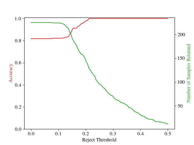
The Reject Option (10 points)
The averaged predictions obtained via Monte Carlo integration are attractive in that we have well-defined probabilities. This provides us with a reject option: if the model is not sufficiently confident about a prediction, it can choose to not predict its class label.
To better understand this, you will run the model under such a reject option. Namely, for a specific threshold (e.g. in the range [0,0.5]), you should perform the following:
- Gather all samples in the test dataset whose highest predicted probability, over all classes, exceeds the threshold. Interpret this as all samples we are willing to predict, given the threshold.
- For this subset of samples, compute the accuracy on the ground truth.
For a series of thresholds, you will then plot the above 2 quantities - number of samples retained, and their accuracy - on the same graph, both as line plots. You should do this for different training data sizes, which you may obtain by simply selecting data in the training set uniformly-at-random, without replacement. The number of training data subsets, and their sizes, are left to you to decide.
In the end, this will provide us with a series of plots. In your write-up, you should include these plots, accompanied with a discussion. What are your findings? What happens with our reject option when the number of training data samples increases?
As an example plot, please see the following image (number of training data samples omitted intentionally):
Suggestions
- Start simple: work off of the
simple_tester.pyscript first. The data is small enough that you can implement Newton’s method by inverting the Hessian directly, without needing to apply the Woodbury matrix identity. And, you can see your resulting model’s prediction. Once you are confident that everything is correct, then you can move on to the more scalable implementation. - This assignment should not require too much code to write. Before sitting down to code, you should think carefully about how to approach each aspect of the assignment. If you are experienced with NumPy, and comfortable using batch-based matrix multiplication, then many of the operations that you need to perform are relatively straightforward. Otherwise, for efficient block-structured matrix operations, it will be necessary to carefully organize your matrix structures.
Appendix
Here I list mathematical details necessary to compute the Hessian in a scalable manner, essentially replicating what we discussed during lecture, but including it here as a single point of reference.
Recall that we aim to compute the following:
$(K^{-1} + W)^{-1}$,
where $K$ is the block-structured covariance matrix of size $\mathbb{R}^{(n \cdot c) \times (n \cdot c)}$ for $n$ training data instances and $c$ class labels, and $W$ is the Hessian of the softmax, of the same size. We note that this is the negative of the log posterior Hessian, which is actually what is used in Newton’s method.
Now, we can write the matrix $W$ as:
$W = \textbf{diag}(\mathbf{\pi}) - \Pi \Pi^T$.
In the above, $\mathbf{\pi}$ is a vector of size $\mathbb{R}^{n \cdot c}$ that contains the softmax values over all data items and classes, and $\textbf{diag}(\mathbf{\pi})$ forms a $\mathbb{R}^{(n \cdot c) \times (n \cdot c)}$ diagonal matrix with $\mathbf{\pi}$ on its diagonal.
The other matrix, $\Pi$, is of size $\mathbb{R}^{(n \cdot c) \times n}$, which vertically stacks a total of $c$ different $n \times n$ diagonal matrices, each one specific to a class that contains the softmax values $\mathbf{\pi}$ for all data items.
Now, to utilize the Woodbury matrix identity, we first decompose the above in terms of the following:
$(K^{-1} + W)^{-1} = (K^{-1} + \textbf{diag}(\mathbf{\pi}) - \Pi \Pi^T)^{-1} = (A - \Pi \Pi^T)^{-1}$,
where $A = K^{-1} + \textbf{diag}(\mathbf{\pi})$. From here, we apply the Woodbury matrix identity:
$(A - \Pi \Pi^T)^{-1} = A^{-1} - A^{-1} \Pi (\Pi^T A^{-1} \Pi - I)^{-1} \Pi^T A^{-1}$.
A few notes:
- The matrix $A$ is block-structured. Thus, we need only compute its inverse on the individual blocks, one matrix per class.
- The inner matrix $(\Pi^T A^{-1} \Pi - I)^{-1}$ is of size $\mathbb{R}^{n \times n}$, and thus efficient to compute.
Now, we never need to compute this explicitly. We only need to compute matrix-vector products with this inverse matrix, and thus, one-by-one we can compute these products from right-to-left.
You will find this necessary for Newton’s method, in addition to forming the predictive covariance.